In Review...
In AppSheet & FRC: Episode 4, I showed how to use three powerful formulas: =ARRAYFORMULA, =VLOOKUP, and =QUERY. We also reviewed some simple use cases in a sample database to grasp how each formula operates.
Now that we have a base of knowledge regarding each formula, it’s time to put that knowledge into practice and start designing a system of analysis for the data collected by our scouters.
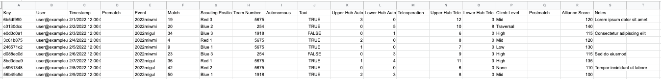
Since we haven’t touched Google Sheets since Episode 2, the screenshot below shows the layout of the columns we’re using based on how we designed things in AppSheet. Since then, I’ve added a few rows of sample data to demonstrate this episode’s work better.
What Do We Analyze?
The first point to consider when designing our analysis tools is what we should be analyzing. We want data on each team competing at our current competition, but what data do we want on them? The answer to this question will vary greatly year-to-year and depends on what qualities you value in other teams. For this exercise, though, I’ll demonstrate how to calculate each robot’s average score—the total number of points a given team has scored divided by the number of matches they’ve participated in.
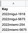
However, to calculate this statistic, we need a list containing each robot in our dataset. Specifically, since we don’t want to aggregate a robot’s score across multiple competitions,1At least not for this exercise. we need a list of each unique combination of event and robot that we have data on. To calculate this, we can use the following formula:
=SORT(UNIQUE(ARRAYFORMULA(IF(ISBLANK('Match Scouting'!A2:A),,'Match Scouting'!E2:E&"-"&'Match Scouting'!H2:H))),1,TRUE)In the screenshot on the right, the E column is the Event column, and the H column is the Team Number column. These two columns are concatenated with a dash in between, creating a unique way of referring to each combination of event and team number. =IF and =ISBLANK are used to replace the result of the concatenation with a blank entry if column A, the Key column, is empty. =ARRAYFORMULA is used to ensure the formula is applied to the entirety of the columns it references and =UNIQUE removes any duplicate values. Finally, =SORT makes the list alphabetical, which will be relevant later.
Note that since I’m doing this analysis in a new sheet, referencing our dataset also requires providing the name of the sheet in single quotes followed by an exclamation mark.
The result is a column where every combination of Event and Team Number is represented, but no combination is duplicated. Our goal now is to calculate the average points for each combination in the list.
Calculating Point Values
Of course, to calculate the average points each team has scored, we first need to calculate the total number of points each team has scored. This can be done with the following formula:
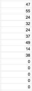
=ARRAYFORMULA(IF('Match Scouting'!J2:J,2,0)+'Match Scouting'!K2:K*4+'Match Scouting'!L2:L*2+'Match Scouting'!N2:N*2+'Match Scouting'!O2:O+SWITCH('Match Scouting'!P2:P,"Low",4,"Mid",6,"High",10,"Traversal",15,0))Column J contains a true/false value representing whether the robot Taxied in the given match, so =IF is used to provide a score of 2 or 0 as appropriate. Columns K, L, N, and O contain how many pieces of Cargo the robot scored in various categories. The values in these columns are multiplied by constants based on how many points each category is worth. =SWITCH is used on column P to provide varying points depending on what climb the robot completed, defaulting to 0. Finally, all of these values are summed together and wrapped in =ARRAYFORMULA.
As seen on the left, this creates a column of values calculating the number of points scored by a robot in each match. These results are in the same order as the rows in the original table. The series of 0s2The 0s continue down the column indefinitely. are from empty rows.
Creating a Query
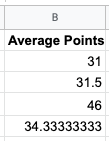
Now that we have an array of point values, we need to aggregate them for each unique combination of robot and competition. This is a perfect job for =QUERY. The following formula will do what we need:
=QUERY(ARRAYFORMULA({IF(ISBLANK('Match Scouting'!A2:A),,'Match Scouting'!E2:E&"-"&'Match Scouting'!H2:H),IF('Match Scouting'!J2:J,2,0)+'Match Scouting'!K2:K*4+'Match Scouting'!L2:L*2+'Match Scouting'!N2:N*2+'Match Scouting'!O2:O+SWITCH('Match Scouting'!P2:P,"Low",4,"Mid",6,"High",10,"Traversal",15,0)}),"select avg(Col2) where Col1 is not null group by Col1 label avg(Col2) ''") This takes the result of our earlier point-calculation =ARRAYFORMULA, along with a second column containing the concatenated results of columns E and H. It then finds the average number of points scored for every combination of team number and event, only including those rows where the Key column has a value and leaving off the default labels. Note that =QUERY automatically sorts the results based on the group by column.3This cannot be relied on in all software, but Google Sheets explicitly states this is the case in its Query Language Reference. This means that it will automatically line up with the results of =UNIQUE from earlier because both are in alphabetical order.
Going Beyond
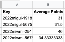
The final result of our formulas is shown on the left, with the =SORT(UNIQUE([...] formula in A2 and the =QUERY(ARRAYFORMULA([...] in B2.4The =ARRAYFORMULA(IF([...] is only used as a sub-formula and doesn’t appear in our final result. Similar formulas can be used to calculate other relevant statistics. A few examples are shown below, along with the analysis each generates using my sample data.
Alliance Carry Percentage
One statistic that 5675 found very useful during the 2022 season was something we called “Alliance Carry Percentage.” This statistic answers the question: on average, how much of their Alliance’s score does a team account for? We noticed that some teams were ranked lower than they should have due to bad luck with their Alliance partners. Alliance Carry Percentage highlights those teams by focusing not on the total amount of points they scored but on how well they did relative to their teammates.
Note that the screenshot on the right shows the results of the formula below formatted as a percentage, which can be done by selecting the C column and then clicking More formats > Percent, as shown in the below-right screenshot.
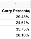
=QUERY(ARRAYFORMULA({IF(ISBLANK('Match Scouting'!A2:A),,'Match Scouting'!E2:E&"-"&'Match Scouting'!H2:H),{IF('Match Scouting'!J2:J,2,0)+'Match Scouting'!K2:K*4+'Match Scouting'!L2:L*2+'Match Scouting'!N2:N*2+'Match Scouting'!O2:O+SWITCH('Match Scouting'!P2:P,"Low",4,"Mid",6,"High",10,"Traversal",15,0)}/'Match Scouting'!R2:$R}),"select avg(Col2) where Col1 is not null group by Col1 label avg(Col2) ''")When interpreting the results of the Alliance Carry Percentage column, keep in mind that a score of 33.33% should be considered standard, with a higher or lower percentage than that indicating an above- or below-par team, respectively.
Taxi Percentage
As the name suggests, the Taxi Percentage for a team represents the percentage of matches where they managed Taxi during autonomous. Although this statistic became less valuable as the season wore on and the quality of robots improved,5 Nearly all teams’ Taxi Percentage approached 100% toward the end of the season. it was helpful during 5675’s first competition to see which teams had a functioning autonomous program.
=ARRAYFORMULA(IF(ISBLANK(A2:A),,COUNTIFS(IF(ISBLANK('Match Scouting'!A2:A),,'Match Scouting'!E2:E&"-"&'Match Scouting'!H2:H),A2:A,'Match Scouting'!J2:J,TRUE)/COUNTIF(IF(ISBLANK('Match Scouting'!A2:A),,'Match Scouting'!E2:E&"-"&'Match Scouting'!H2:H),A2:A))) 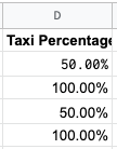
Total Cargo
Although the number of points a team scores is usually the more practical statistic, sometimes it can be helpful to know how many game pieces a team scores. The formula below calculates the average total amount of Cargo a team scores, combining the autonomous and teleoperation periods.
=QUERY(ARRAYFORMULA({IF(ISBLANK('Match Scouting'!A2:A),,'Match Scouting'!E2:E&"-"&'Match Scouting'!H2:H),'Match Scouting'!K2:K+'Match Scouting'!L2:L+'Match Scouting'!N2:N+'Match Scouting'!O2:O}),"select avg(Col2) where Col1 is not null group by Col1 label avg(Col2) ''") 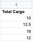
Cycle Time
A team’s Cycle Time is how long it takes that team to go from scoring one piece of Cargo to scoring the next. This value is equal to the number of seconds in the teleoperation period of a match6In 2022, as in most years, teleoperation lasted 135 seconds. divided by the amount of Cargo the team scores during that time.
=ARRAYFORMULA(135/QUERY(ARRAYFORMULA({IF(ISBLANK('Match Scouting'!A2:A),,'Match Scouting'!E2:E&"-"&'Match Scouting'!H2:H),'Match Scouting'!N2:N+'Match Scouting'!O2:O}),"select avg(Col2) where Col1 is not null group by Col1 label avg(Col2) ''")) 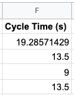
What Next?
After this episode, most of the work is done. We’ve built an app that can collect data on our opponents, piped the data into Google Sheets, and developed advanced analytical tools that sift out crucial insights.
In the next and final episode, I’ll show how to generate a professional-style report showcasing our analysis. I’ll also explain how to utilize Google Sheets’ built-in interface for designing graphs and charts, adding visual impact to the presentation of our data.