In AppSheet & FRC: Episode 5, I explained how to use advanced Google Sheets formulas to analyze our data. This included the process of determining what to analyze, calculating various valuable statistics, and then associating the final results with the targets of our analysis.
Currently, though, it’s a bit unwieldy to look at our analysis. The examples from the last episode only had a few rows, but there will be many teams at an actual competition. It’s imperative that we have a method for trimming down our results into something that’s more user-friendly, which is the focus of this episode. Furthermore, during competitions, having a paper copy of the analysis is often beneficial, so I’ll also explain how to create an easily-printable version of our results.
Layout
Fortunately, Google Sheets has built-in functionality for directly printing a sheet or subsection thereof. Once we put our data into a format easily readable by a human, no further work is needed before it can be directly printed. However, this means that as we create the layout for our data, we should think about how it will ultimately be printed.
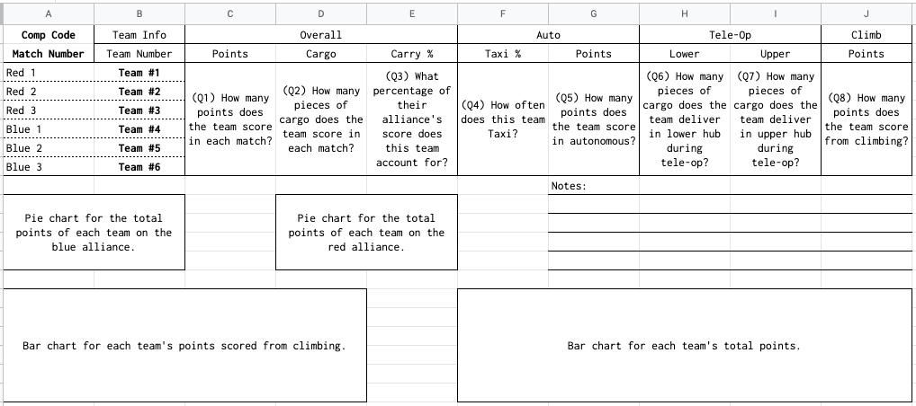
In this case, I will show how to create a report that roughly matches the layout below. This will make for convenient landscape-style printing. Of course, alternative layouts are possible.
The goal is that the user will fill in the Comp Name, Match Number, and Team Number fields (in bold), and the answer to all eight questions will be automatically populated using formulas. During the last episode, I explained how to calculate the statistics for Q1 through Q4, with the remaining ones explained below. Also, note the dedicated space for four charts and an extra area for providing hand-written notes after printing.
Additional Formulas
Q5
=QUERY(ARRAYFORMULA({IF(ISBLANK('Match Scouting'!A2:A),,'Match Scouting'!E2:E&"-"&'Match Scouting'!H2:H),'Match Scouting'!K2:K*4+'Match Scouting'!L2:L*2}),"select avg(Col2) where Col1 is not null group by Col1 label avg(Col2) ''")
Q6
=QUERY(ARRAYFORMULA({IF(ISBLANK('Match Scouting'!A2:A),,'Match Scouting'!E2:E&"-"&'Match Scouting'!H2:H),'Match Scouting'!O2:O}),"select avg(Col2) where Col1 is not null group by Col1 label avg(Col2) ''")
Q7
=QUERY(ARRAYFORMULA({IF(ISBLANK('Match Scouting'!A2:A),,'Match Scouting'!E2:E&"-"&'Match Scouting'!H2:H),'Match Scouting'!N2:N}),"select avg(Col2) where Col1 is not null group by Col1 label avg(Col2) ''")
Q8
=QUERY(ARRAYFORMULA({IF(ISBLANK('Match Scouting'!A2:A),,'Match Scouting'!E2:E&"-"&'Match Scouting'!H2:H),SWITCH('Match Scouting'!P2:P,"Low",4,"Mid",6,"High",10,"Traversal",15,0)}),"select avg(Col2) where Col1 is not null group by Col1 label avg(Col2) ''")
Autofilling Data
The formulas above should answer all eight questions, but work is still needed to get their results into our new formatted layout. This is a situation that requires the use of the =VLOOKUP formula. Utilizing the user-provided fields for the competition code and team number, we can search through the table we created in the last episode for each question’s answer.
For example, the formula in cell D3 would be the following:1Assuming that your “Total Cargo” column from the last episode is column E in a sheet named “Team Reports”.
Note the use of the =IFERROR function. This allows for the possibility that the team in question has not yet played any matches at the current competition, in which case, the displayed value will default to 0.
As another example, the formula in cell F6 would be the following:
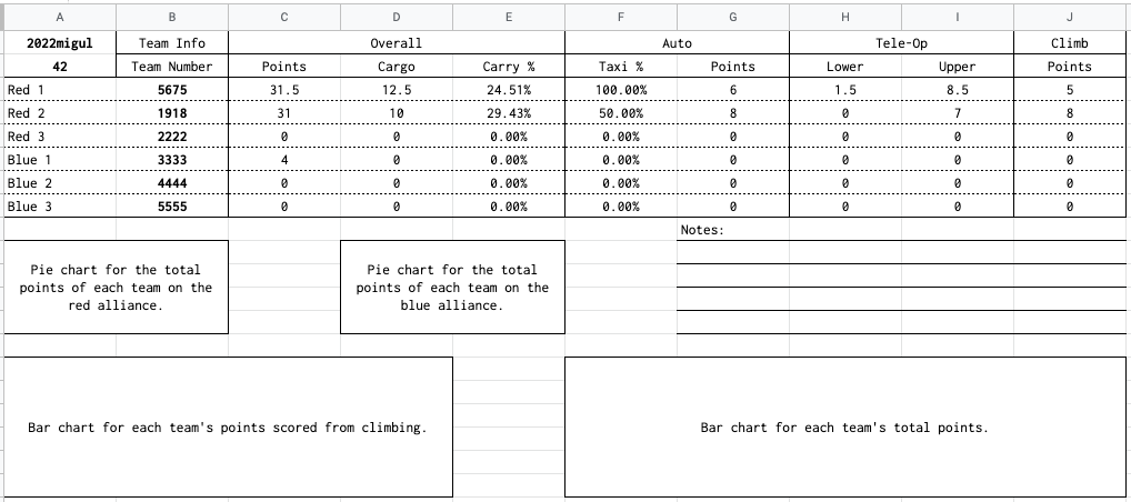
After applying appropriate formatting to all cells, your results should be similar to the screenshot below.
Creating Charts
Pie Charts
We now have numerical information on each user-provided team, but it’s still not presented in the most user-friendly way. Using charts, we can make it much easier to parse the provided statistics at a glance.
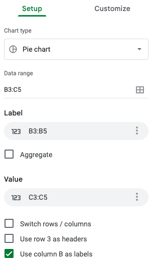
Let’s start with the pie chart for the red alliance. In the top bar, click on Insert > Chart. Change Chart type to be Pie chart. Set a Data range of B3:C5. Set Label to be B3:B5 and Value to be C3:C5. The Chart Editor screen should look similar to the screenshot on the top right.
The following are some recommended changes in the Customize section that can make the chart clearer to read once printed:
Chart style > Font: Courier New
Chart style > Chart border color: black
Pie chart > Border color: black
Pie chart > Slice label: Percentage
Pie chart > Label font: Courier New
Pie chart > Label format: Bold
Pie chart > Text color: black
Pie slice > Pie slice selector > [Slice 1] > Color: dark gray 3
Pie slice > Pie slice selector > [Slice 2] > Color: dark gray 1
Pie slice > Pie slice selector > [Slice 3] > Color: light gray 1
Chart & axis titles > Title type selection > Chart title> Title text: Red Alliance
Chart & axis titles > Title type selection > Chart title> Title font: Courier New
Chart & axis titles > Title type selection > Chart title> Title format: Bold
Chart & axis titles > Title type selection > Chart title> Title text color: black
Legend > Position: Left
Legend > Legend font: Courier New
Legend > Legend format: Bold
Legend > Text color: black
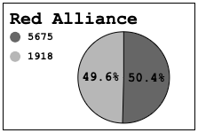
If you apply the above formatting changes, the result should look similar to the screenshot on the bottom right. If you added sample data for a third team at whichever competition you’re testing, data on them should also appear.
You can use similar steps to create the chart for the Blue Alliance, operating on B6:C8 instead of B3:C5.
Bar Charts
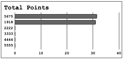
Making a bar chart requires a similar process. Insert a new chart and change its type to be a Bar chart, taking a data range of B3:C8. Set the X-axis to be B3:B8, and add a single Series for C3:C8. Using similar customization options to the ones described for a Pie Chart, you should end up with something similar to the below-left screenshot.
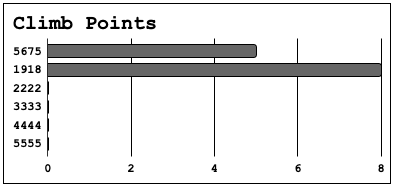
To make a bar chart for climb points, use two ranges: one from B3:B8 and another from J3:J8. Make sure that Combine ranges is set to Horizontally. You should end up with something similar to the above right screenshot.
The Final Result
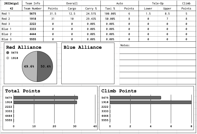
The final result of our efforts2After some slight resizing of columns and rows. is shown in the below screenshot. Alternatively, press the button on the right to see the result as a PDF.
If you have additional sample data, the rest of the rows will be filled out, and your charts will look much less sparse.