AppSheet & FRC: Episode 4

In Review...

In AppSheet & FRC: Episode 3, I showed how to make some UI updates in AppSheet, creating a smoother experience when scouters input data into the app. I also showed methods for error-checking, introducing requirements and limits, then finished with an explanation of the Principle of Least Privilege.

Now that things in AppSheet are solidified and polished, it’s time to switch to Google Sheets and work on methods for analyzing our data. In this episode, we’ll depart from our primary dataset to work on a smaller and more approachable series of examples. This will build the conceptual understanding needed to apply complex formulas to our fullscale dataset.

Three Major Formulas

During this episode, I will explain three powerful formulas crucial to our later work. These three formulas are =ARRAYFORMULA, =VLOOKUP, and =QUERY. All three are robust tools for creating dynamic and scalable composite Google Sheets formulas, allowing for powerful analysis of our data.

=ARRAYFORMULA

The first of our three functions is =ARRAYFORMULA. As its name suggests, it assists with the processing of arrays,¹ having two primary use cases:

It allows formulas that return arrays to display their results in full.
It allows formulas not built for handing arrays to be used with arrays.

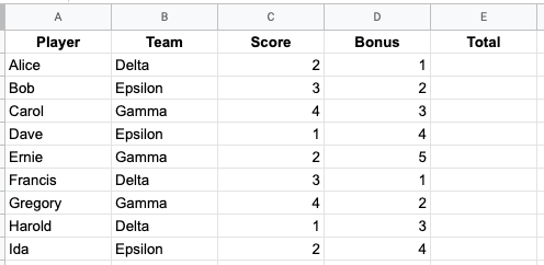
Let’s say we’ve got data on a game where there are two ways for players to score points: scoring normally or earning bonus points. We want to calculate the total score each player has achieved.

One method of doing this would be to put a separate formula² in each row of column E. This is a serviceable way of doing things, but it has two issues:

If we add more players to the data set, we will have to add a formula to the next row each time it happens.³
If the way we calculate points changes—if bonus points are doubled, for instance—we will have to change the formula for every row.

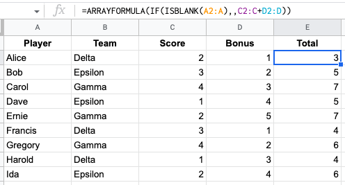
However, through the power of =ARRAYFORMULA, we can improve our methods. With it, we only need to write one formula that automatically fills in the information we want into the entire E column. In this case, putting the formula =ARRAYFORMULA(C2:C+D2:D) in cell E2 will do just what we need. You might notice that this also creates a long series of zeros in the extra rows of column E, but this can be fixed by adding a check using =ISBLANK to do the calculation only if column A has a value: =ARRAYFORMULA(IF(ISBLANK(A2:A),,C2:C+D2:D)).

Now, our two problems are resolved. Adding new rows to the data set doesn’t necessitate changing anything because that’s automatically taken care of for us. Furthermore, if we ever decide to change how the total score is calculated, we only have to modify a single formula rather than an entire column.

=VLOOKUP

Now that we’ve calculated the total score for each player, it would be nice to have a more convenient way to find that information. Currently, if we want to know how well a given player did, we would have to look through our raw data to find that out. This is manageable for now, but imagine a situation where we have thousands of players: things would quickly get intractable.

This is where =VLOOKUP comes in. It allows us to tell Google Sheets a value to look for in a particular column and then find other information about the row where that value is found. In the example below, we use =VLOOKUP to find the row for a specific player (in this case, Francis), then find that player’s total score.

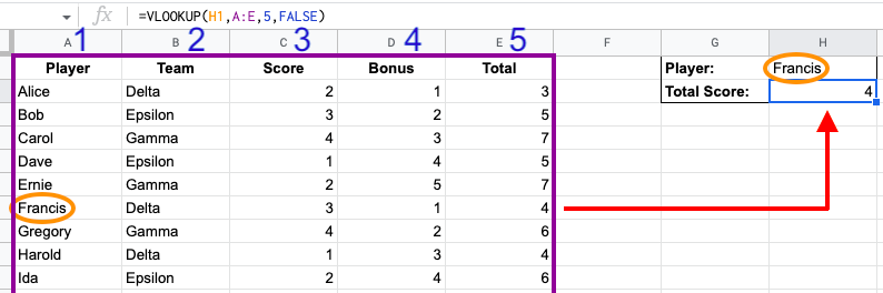
There are four parts to =VLOOKUP syntax:

The search key. In this case, the value in H1.
The range to search through. In this case, columns A through E are used.
The index of the value to return. This starts counting at 1 with the leftmost column in the range and increases moving right.
The is_sorted parameter. For our purposes, the last parameter of =VLOOKUP should always be FALSE.

=VLOOKUP works by attempting to find the search key in the first column of the range. When it finds the value, it checks the index to see which column of the range should be returned. The natural limitation is that the column to be returned must be to the right of the column to search through.

Furthermore, if the search key is not a unique value, =VLOOKUP might not return the value we want. That’s why it’s crucial that =VLOOKUP is only used on key columns—that is, columns that are guaranteed to contain a unique value in each row. In an actual application, using someone’s name as a search key would be a terrible idea since there could easily be multiple people with the same name, but it’s okay for this example.

=QUERY

Through the previous two formulas, we have methods by which we can calculate our data and then retrieve individual entries. But something’s still missing—we cannot retrieve aggregate information from our data set. This is where =QUERY shines. It allows the extraction of information from a dataset that considers multiple entries (such as averages, maximums, and minimums) and has provisions for sorting and grouping the results.

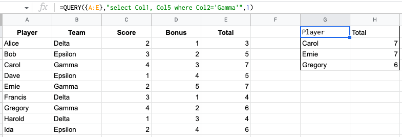
Let’s say we want to see information on all players who are part of team Gamma and their total scores. =VLOOKUP would be cumbersome for this, requiring six separate formulas. Fortunately, =QUERY provides a much easier way, as shown in the example below.

There are three parts to =QUERY syntax:

The data. In this case, columns A through E are used.
The query. This is a string surrounded by double quotes that describes what operations to perform on the data.
The headers. This states how many header rows there are in the data. In this case, row 1 (in bold) is a header row, and everything below that is actual data.

=QUERY works by evaluating the query, running the described operations on the data, and then returning the result as an array. In the example above, the query selects only columns 1 and 5 to be returned in the result, discarding the Team, Score, and Bonus columns. Then, it checks each row and only returns those where the player’s Team is Gamma. Finally, it automatically adds the header values for the two columns it returned: Player and Total.

That’s a convenient way to gather information on a subset of rows. As mentioned earlier, we can also find aggregated information about multiple rows, such as checking how many total points each team scores on average. For example, Bob, Dave, and Ida are all on the Epsilon team, and their average score is 5.33.⁴In the example below, we use =QUERY to find the average total score for each team.

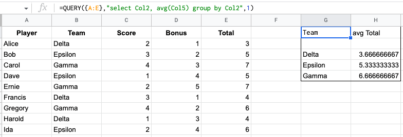
The query selects only columns 2 and 5 to be returned in the result, discarding the Player, Score, and Bonus columns. Then, it divides the data in column 5 into three groups based on the value of column 2 and takes the average of each group. Finally, it automatically adds header values, guessing at what we would want the average of Total to be called.

However, the way the result is currently formatted is slightly awkward. avg Total isn’t a very intuitive name. There’s also a weird extra blank row, which is generated because =QUERY actually makes an additional fourth group for values in column 2 which are null, or in other words, empty. These problems are fixed in the example below.

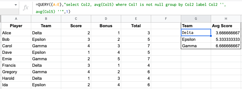
In the example above, the query selects only columns 2 and 5 to be returned in the result, discarding the Player, Score, and Bonus columns. It also ignores any column where the value of column 1 is null. Then, it divides the data in column 5 into three groups based on the value of column 2 and takes the average of each group. Finally, the labels for column 3 and column 4 are both set to be empty, meaning that =QUERY doesn’t bother automatically adding header values.⁵

What Next?

At this point, you should have a solid conceptual understanding of =ARRAYFORMULA, =VLOOKUP, and =QUERY. Don’t worry if you aren’t confident regarding the syntax yet; I’ll be walking through further examples in future episodes. That said, if you’re interested, =QUERY is fully documented in Google’s Query Language Reference.

In the next episode, I’ll return to the full-scale dataset our app is built for. Once we’re reacquainted with it, I’ll then show how to use all three formulas from this episode in concert to automate our data analysis.